Note: There was no reading assigned for this lecture. This is post-class material covering the topics we didn’t get to.
During the lecture, our goal was to cover three topics, but we only managed to address the first one. Below is an outline of the first topic covered, along with reading notes for the remaining two.
Routing on the Internet, BGP
In the lecture, we explored the following:
- Topology of the public IPv4 Internet.
- The necessity for unique IP addresses within a network.
- IPv4 address assignment flow (IANA -> RIRs -> ISPs -> end users).
- Hierarchical structure of IPv4 addresses (illustrated through a block subdivision example).
- Example scenario: interconnected routers with their routing tables.
- Comparison between directly connected device routes and regular routes with specified gateways (with via keyword).
- Discussion on static versus dynamic routing for exchanging routing information.
- Explanation of dynamic routing protocols handling the job versus the IP protocol forwarding IP packets based on the routing table.
- Overview of routing protocols such as RIP, OSPF, and BGP.
- Introduction to routing daemons, specifically BIRD.
- Autonomous Systems (ASes) on the Internet, Autonomous System Numbers (ASNs) in the context of BGP.
- BGP, including its use of TCP port 179, the AS path as a criterion for determining the shortest path, and its role in loop detection, eBGP vs. iBGP.
- Examination of the BIRD architecture, emphasizing concepts like internal routing tables, protocols, and channels. Device, kernel and direct pseudo-protocols. channels, including pseudo-protocols like device, kernel, and direct.
- BIRD configuration example: Three routers connected through one common backbone network (10.0.0.0/24). Two routers in addition connected to two stub networks each (the first to 10.1.1.0/24 and 10.1.2.0/24, the second to 10.2.1.0/24 and 10.2.2.0/24). All routers running BIRD and peering via the middle router using BGP. Without BIRD, we were not able to reach one stub network from the other because the routes to the destination network were missing. This changes after running BIRD.
IPv4 address space exhaustion
The IPv4 protocol, conceived in the late 1970s, saw its first standard published in 1980. As the Internet witnessed unprecedented growth in the latter half of the 1980s, fueled by the widespread availability of connectivity through dial-up connections over telephone wires, the number of end users surged significantly. In an IP network, each node must be uniquely identified by its IP address. By the end of the 1980s, it became evident that the global IPv4 address range, totaling 2^32 (4,294,967,296) addresses, would not be sufficient to identify every individual node in the near future, and the exhaustion of the global range was inevitable.
To mitigate this impending exhaustion, several mechanisms were introduced to at least delay the issue:
-
CIDR Subnetting Scheme (1993): The Classless Inter-Domain Routing (CIDR) subnetting scheme replaced the earlier class-based subnetting scheme in 1993. The class-based scheme was rigid and led to inefficient IP assignments. CIDR brought flexibility by allowing more efficient allocation of IP addresses based on actual needs. Unlike the class-based scheme, where companies were assigned the nearest larger block, CIDR facilitated more precise allocations, reducing unused IP addresses.
-
Private Address Ranges (1994 and 1996): In 1994, RFC 1597 introduced private address ranges, preceding the widespread adoption of CIDR. In 1996, RFC 1918 replaced RFC 1597 while still leveraging CIDR. The introduction of private address ranges allowed organizations to use non-routable IP addresses within their private networks. Although CIDR made the overall address space more efficient, private IP ranges helped alleviate the strain on public IP addresses.
-
Network Address Translation (NAT) (1994): Before the widespread use of NAT, proposed in 1994, there was a need to address the challenge of “hiding” multiple hosts in a private network behind one device with a public IP. NAT allowed multiple devices in a private network to share a single public IP address, helping to conserve the limited pool of public IP addresses.
These three events played a crucial role in shaping the evolution of the Internet, influencing its current structure. While the transition from the class-based scheme to CIDR is considered a positive design choice, the same cannot be said for the latter two mechanisms. Now, let’s delve into more detail about them.
Before we do, it’s important to note the conclusion of the story concerning IP exhaustion. Unfortunately, the measures taken did not fully address the issue. On January 31, 2011, the IANA central authority assigned the last two blocks to APNIC RIR, making APNIC the first Regional Internet Registry (RIR) to run out of IP addresses. Subsequently, on November 25, 2019, RIPE became the last RIR to exhaust its pool of available IP addresses. Although IPv4 addresses are still owned by ISPs redistributing them between their customers, the scarcity persists. Over time, as customers leave or ISPs dissolve, IP addresses are returned to the corresponding RIRs. At the RIR level, there exists a waiting list of applicants seeking IP address blocks. While it is still possible to request public IPv4 addresses or blocks, they are now considered valuable and relatively expensive commodities.
Public vs. Private IP Addresses, NAT
If you are operating an isolated network where devices are interconnected without any external connection, you have the freedom to use any IP address range, and it will function seamlessly. No one is required to allocate specific blocks, granting you the flexibility to choose an arbitrary range. However, potential issues may arise if, at a later stage, you decide to connect to the public Internet or integrate with another corporate network, especially in the case of mergers. The challenge lies in the necessity for unique IP addresses, and using an arbitrary range is considered bad practice. Instead, it is advisable to employ an IP range assigned by the corresponding authority (RIR or ISP) or utilize a specially designated private range.
In 1994, before the introduction of RFC 1597, there was no dedicated private range. All IPs were considered global (or public) IPs, lacking the distinction present today. RIRs and ISPs globally assigned IPs without differentiation, contributing significantly to the problem of IP exhaustion.
Originally designed to route the Internet, the IP protocol gained popularity and found application in “private” setups. Institutions, such as universities, were assigned blocks of public IP addresses for widespread use, even on devices like workstations in university libraries and printers. It became evident that these devices did not require a globally routable (public) IP address, as it was unlikely that anyone outside the university would need to access these devices over the Internet. In response, private IP ranges and Network Address Translation (NAT) were introduced.
RFC 1918 reserved three blocks of the global IP address range for use in private networks:
- 10.0.0.0 - 10.255.255.255 (10/8 prefix)
- 172.16.0.0 - 172.31.255.255 (172.16/12 prefix)
- 192.168.0.0 - 192.168.255.255 (192.168/16 prefix)
These reserved blocks are not assigned to anyone else on the Internet. The key concept here is that IP addresses from these ranges can be reused by an infinite number of private networks that do not require “global” connectivity, thereby conserving global address space. However, this reuse seemingly contradicts the requirement for unique IP addresses across the Internet.
In a world with private ranges, the Internet transforms from a single, massive network into a global one, with addresses assigned as usual and numerous private stub networks somehow connected to the larger Internet. To maintain functionality, a thick boundary must be established between the private network and the rest of the Internet. Inside a private network, IP addresses are assigned uniquely, avoiding clashes with other devices in the same private network. However, clashes with someone else’s private network are possible, but due to the thick boundary, direct connectivity between private networks over the global Internet is lost – a trade-off that must be accepted.
It’s worth noting that subnetting within the private range is possible. For instance, using the 10.0.0.0/8 prefix for addressing a private network allows further subdivision into several subnets (e.g., 10.1.0.0/16 and 10.2.0.0/16), enabling the use of different subnets for various departments within a company.
Ensuring that these private ranges are reserved and not used by anyone else on the Internet is crucial. Using an unreserved arbitrary range for numbering a private network may work if you are fortunate, but it could also lead to clashes with other entities on the Internet. In such a scenario, the Internet would still function, but you would be unable to reach the intended target. For example, choosing to use the 1.1.1.0/24 range for a private network could result in conflicts, such as a user attempting to visit the CloudFlare website https://one.one.one.one/ (with an IP of 1.1.1.1). The user’s PC would believe that 1.1.1.1 is reachable in the local network, causing the connection to fail.
The concept of the “thick boundary” raises the question of how private networks maintain connectivity with the global Internet. This is where NAT comes into play.
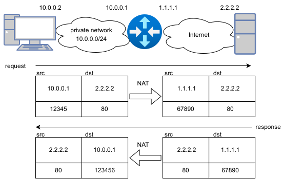
NAT, or Network Address Translation, is a technique for altering network headers, primarily IP, TCP, or UDP headers, of packets in transit. Commonly, the altered parameters include src/dst IP addresses and src/dst port numbers. When altering source parameters, it is known as SNAT or SRCNAT, and when altering destination parameters, it is referred to as DNAT or DSTNAT.
NAT is typically deployed on a boundary router in a private network, which also has a public IP assigned to one of its interfaces. If SNAT is deployed on such a gateway, it can “hide” the network behind its public IP address, a process known as masquerading. When a packet arrives at the gateway, the original source address of the packet is replaced with the gateway’s public IP. The packet is then routed to the destination as usual. When a response is sent back, the original source IP becomes the destination. The response is sent to the globally routable IP address of the router, where the NAT mechanism translates the destination IP back to the original sender’s address. However, this introduces a challenge: if multiple PCs in the private network request the same server and two responses arrive at the router, the router needs to distinguish to which host it should forward the response. This is why NAT also changes port numbers in the TCP/UDP headers.
The workflow of this situation is as follows:
- When a packet is sent by the sender, a random free port is used as the source port, and the sender’s IP address is used as the source address.
- When the packet reaches a NAT gateway, SNAT changes the source address as described. Simultaneously, it changes the original source port to another random free port and maintains a NAT table. An entry is added to the table stating: “The original source IP address and source port correspond to this changed port.”
- The packet is routed to the destination.
- At the destination, the reply is sent to the sender, and source IP and ports become the destination.
- The packet is routed back to the NAT gateway.
- On the gateway, the NAT table is looked up, and based on the destination port (which was the altered source port before), the destination address and port are translated back to the original.
- The packet is routed to the original sender in the private network.
It’s important to note that the example above illustrates SNAT. Even if the flow in the opposite direction could be perceived as DNAT, it is not DNAT; it’s the second complementary part of SNAT. The initiator determines whether it is SNAT or DNAT.
Also, masquerading is just one of many NAT usage examples. For instance, DNAT can be used for port forwarding from a public IP to a private IP, enabling a host inside a private network to be reached through the NAT gateway. Further tasks related to this will be discussed.
In summary, the complex interplay between private and global networks, along with the introduction of NAT, has significantly shaped the contemporary landscape of network addressing and connectivity.
nftables (filter and NAT)
For further understanding and practical application, refer to the following links:
Here are some useful links which should help you to grasp the topic and mostly the practical aspects:
- Firewall in general – What it is and why is it useful. For more reasoning, see task description in evalweb.
- What is nftables? – In basic words: firewall and NAT implementation for Linux. Successor of former iptables.
- Quick reference-nftables in 10 minutes – This should help you to find out how to configure nftables. Only filter and nat table types and ip family should be relevant for you.
- This diagram can be useful to understand how hooks work and what is the packet flow on Linux. Only the first top layers should be relevant for you (orange and green rectangles).