This text covers very basic networking topics. It focuses exclusively on Ethernet, IP and their implementation in Linux. It is not a replacement for a full course, such as NSWI090. Rather, it should help us establish some common ground upon which we can build.
Encapsulation
Practical networks use a layered approach: rather than having a single technology deliver data from one end to the other, there’s a bunch of protocols stacked on top of each other to get the job done, where the lower layer protocols usually carry the upper layer protocols as payload. For example, IP packets are often carried as payload of Ethernet frames.
Make sure that you grasp this principle called encapsulation in the context of networking. The diagram in Encapsulation (networking) on Wikipedia should make sense to you.
Ethernet
Ethernet is a protocol that operates at the Physical and Link layers and has been with us since the 1980s. The first official standard was released in 1980, but development began even earlier, in the early 1970s. Over the decades, Ethernet has evolved considerably; some components have been altered or discarded, while others have remained unchanged.
Because Ethernet has such a long history, there is a wealth of mostly historical information available. Don’t get me wrong—this information can be fascinating and valuable for history enthusiasts. It shows us the decisions made at crucial points in the development of the technology, the motivations behind those decisions, and ultimately provides insight into why the technology appears as it does today. However, if you’re looking to quickly grasp the key principles, delving into historical details might be more of a hindrance than a help. So, let’s clear away that clutter first:
Ethernet was initially designed around a bus topology. This meant having a single long, thick wire (usually coaxial) running throughout a building. To connect a computer to the network, the cable would be cut, a special T connector inserted, and voilà, you were connected. Being a bus meant that a single medium (the cable) was shared by all machines in the network, with all the consequences: all the traffic was visible to everybody, the machines competed for bandwidth, and collisions would occur when two machines started to transmit at the same time.
For many reasons, this topology was phased out in the 1990s and replaced with twisted pair cabling. One of the reasons for this shift was that twisted pair cabling was often already in place for telephony. So, Ethernet adopted twisted pair, changed its topology to a star (or a tree), and has remained in this state to this day.
Please set aside terms like repeater, hub, collision, collision detection, collision domain, CSMA/CD, etc. They’re all remnants of the distant past. Today, to add devices into an Ethernet network, Ethernet switches (or just switches when Ethernet is implied) are used.
There’s one more term, bridge, which is still in use today, albeit with a slightly different meaning than in the past. You might read online that a bridge was used to reduce the number of collision domains. Technically, that’s true, but let’s not dwell on that. In 2023, collision domains are a thing of the past. Today, a bridge is more or less synonymous with a switch. In terms of functionality, they are essentially equivalent. Typically, switch is used when referring to the physical hardware, and switching is performed in hardware, ensuring high speed. Conversely, bridge is used when the same functionality is emulated in software (e.g., by your operating system). This tends to be slower, but with the processing power of current CPUs, it’s not a significant concern (depending on the use-case). But that’s the only distinction between the two terms these days.
By the way, Ethernet messages are called frames, and the Ethernet header follows this format (taken from Ethernet frame on Wikipedia):
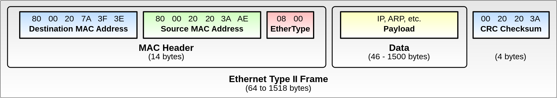
Another crucial aspect that has persisted to this day is Ethernet addressing. Ethernet employs 48-bit MAC addresses to differentiate between end hosts (computers). Only end hosts possess MAC addresses; intermediate devices (switches/bridges) do not. They work with MAC addresses, reading Ethernet headers of frames passing through them, but switches do not possess MAC addresses of their own. (Unless there is some management web interface running on the switch, which may need to be accessible over the network. Even then, it is used only to configure some advanced features of the switch, the switch does not require a MAC address to perform its primary function—switching between its ports.) Be cautious: routers do have MAC addresses because, from the perspective of Ethernet, they are end devices.
MAC addresses are represented as hexadecimal numbers, with each byte separated by a colon (:) or a dash (-). For example, 00:B0:D0:63:C2:26. MAC addresses are configured by your network card driver, and each network card comes with a pre-set MAC address. It’s crucial that each device in a network has a unique MAC address, or otherwise things can go spectacularly wrong. Achieving and verifying this can sometimes be challenging, especially given the current prevalence of device mobility. To simplify matters and ensure safety, MAC addresses are globally unique. The first 3 bytes are assigned to the vendor of the network card by a central authority known as IEEE (pronounced eye-triple-E), and the remaining 3 bytes are assigned sequentially by the vendor.
(By the way, most network card drivers allow you to change the MAC address, and with virtual Network Interface Cards, such as with QEMU, a random MAC address is generated by default; you can also set your own.)
Apart from this, it’s best to leave behind all historical knowledge about Ethernet. If you want to learn more about how we got here, The world in which IPv6 was a good design makes for a fantastic reading.
Transparent Bridging
Transparent bridging/switching is the technique (or algorithm, if you will) that switches employ to forward frames. We’ll assume Ethernet frames in the following text, but the process is very similar for other protocols as well, e.g., 802.11, more commonly known as Wi-Fi.
Each switch maintains its own forwarding table. Every entry (row) in the forwarding table consists of the following items (columns):
- MAC address
- Port number
- Time-stamp
The semantics of each entry are straightforward: “Host with this MAC address resides behind this port, and this information is valid until the time-stamp expires.”
Now, imagine that an Ethernet frame arrives at one of the switch ports. How does the switch determine which port to forward the frame to? Not surprisingly, the switch consults its forwarding table—it reads the destination MAC address of the frame and looks it up in the table. It then sends the frame out on the corresponding port. That’s all there is to it.
Seems simple, right? But when you first power on the switch, or start a virtual bridge, the forwarding table is initially empty. So, how does the switch populate the forwarding table? This is where it gets interesting. It employs three techniques for this: Learning, Aging and Flooding.
Learning
This is the most straightforward one. When a frame (e.g. with a source MAC address of AA:BB:CC:EE:DD:FF) reaches a switch port (say number 7), the switch immediately records the corresponding entry in the table: “Host with MAC address AA:BB:CC:EE:DD:FF resides behind port number 7.”
Initially, this doesn’t assist the switch in determining where to forward the frame. However, when a reply frame to the original one appears in the future (so that the source MAC address becomes the destination MAC address), the switch will already know where to forward it. Not bad.
Aging
This is where the time-stamp comes in. Aging is an optimization technique aimed at keeping the forwarding table compact and not storing stale records. This was particularly important in the past when switch memory was limited.
With each learning step, the time-stamp of the corresponding entry is pushed further into the future by a fixed interval. This corresponds to the amount of traffic flowing through the switch: if a host with a particular MAC address hasn’t been heard from in a long time, its entry is automatically removed from the table.
Also, if a cable is disconnected from one of the switch ports, the switch removes all entries associated with that port from the table.
Flooding
If the table doesn’t contain an entry with the destination MAC address of the incoming frame, the switch has no choice but to flood the frame to all of its ports. This way, the frame eventually reaches its destination. When flooding, the switch excludes the port from which the original frame arrived.
Failure Modes
Will all of this actually work? What if something goes wrong? What could go wrong? Consider possible (and even impossible) failure modes; we’ll delve further into these during the lecture. Try to answer these questions for yourself:
- Can we expand our network by connecting multiple switches together? Will that work? Is any further configuration required?
- In the flooding step, why does the switch omit the port from which the original frame arrived? Is this a necessity or just an optimization?
- If we connect multiple switches together, are there any topology restrictions we should consider? Why?
- What if someone simply disconnects a cable (connected to a computer on the other side) from one switch and reconnects it to a different switch port? Will the computer still be able to communicate with other computers in the network? How is that possible? What if I reconnect the cable to a different switch (connected transitively to the original switch)?
- What happens if two or more computers in the same network end up with the same MAC address assigned? In other words, what occurs with the frame in the network when someone sends such a frame with that destination MAC address?
- Wait, if switches flood frames under certain circumstances, does that mean that strangers in the network will automatically receive traffic intended for me? Is that acceptable?
IPv4 Subnetting
There are two versions of IP currently in widespread use, IPv4 and IPv6. In this chapter, we only concern ourselves with IPv4, as IPv6 will be the subject of a dedicated lecture.
The Internet Protocol (IP) is the foundation of the internet as we know it. It’s used to route packets between networks, and the collection of all interconnected networks forms the internet.
You probably know what an IP subnet is and that each IP address can be divided into its network part (also known as network ID or network prefix) and its host part (or host ID). But why is it designed this way? The simple answer is that the internet is vast, and you need a way to organize it. So, you break down the immense internet into smaller parts—subnets—to be able to reliably deliver a packet from one end to the other. One of the key features of IP subnetting is its hierarchical nature. In essence, the address structure forms a tree.
You’re likely already familiar with the notation for IP addresses and their subnet masks. The subnet mask indicates the length of the IP address prefix considered the network ID and the suffix, which forms the host ID. In other words, it specifies where in the IP address the subnet ID ends and the host ID begins.
This is the standard way to write an IP address and its mask:
- IP address in decimal: 192.168.1.1
- Mask in decimal: 255.255.255.0
- Mask in binary: 11111111.11111111.11111111.00000000
Note that there are 24 “ones” in the mask. There’s another way to express the same information, known as CIDR notation (pronounced like “cider”), 192.168.1.1/24. That’s what we’ll use throughout this course. Both notations convey the same message: the first 24 bits of the address form the subnet ID, and the remainder is the host ID.
You can obtain the subnet ID from an IP address by applying a binary AND operation to the IP address and its mask, resulting in 192.168.1.0, which is the subnet ID of the above IP address.
The subnet mask is crucial when you’re referring to the subnet to which an IP address belongs. This is particularly important when you assign the IP address to an interface or for routing purposes. However, when you’re simply referring to a remote target, it’s common to omit the mask.
Distinguishing whether two addresses belong to the same subnet is a crucial skill. Why? Because if they do, traffic is directly switched to the target machine. Connecting the two machines to a switch, assigning them IP addresses from the same subnet, is sufficient for them to communicate. This is why bridging/switching is called transparent—it’s transparent to both sides, requiring no further configuration on either end.
Conversely, if two machines belong to distinct networks—meaning their IP addresses don’t belong to the same subnet—you’ll need a router to route traffic between the subnets. In this case, traffic is first switched from a machine to the appropriate router (there may be multiple routers in one subnet, each connected to various other subnets), and then from the router to the other, possibly target, subnet. There might be more than one subnet in between the source and destination subnet, of course. That’s how the internet is structured.
Let’s put this knowledge into practice. Determine which IP addresses belong to the same subnet. Use the network calculator to verify your answers. (Note that the calculator refers to subnet ID as the CIDR base IP). For clarity, there are 7 IP addresses and 4 distinct subnets. Assign each address a subnet ID. The subnet ID assignment establishes an equivalence relation on this set of 7 IP addresses. Based on the subnet ID, decide which IP addresses belong to the same subnet:
- 8.8.8.8/24
- 8.8.8.42/24
- 8.8.8.254/24
- 10.1.2.3/16
- 172.16.0.1/12
- 172.17.0.1/12
- 172.32.0.1/12
It’s worth noting that this definition of equivalence might seem a bit unusual. According to it, it implies that these IP addresses:
- 10.0.0.1/24
- 10.0.0.2/24
- 10.0.1.1/16
belong to the same subnet of 10.0.0.0. It’s debatable whether the subnet mask should be considered in subnet identification or not. If not, all the IP addresses belong to the same subnet of ID 10.0.0.0. If yes, the first two IP addresses belong to the subnet of 10.0.0.0/24, whereas the third belongs to the subnet of 10.0.0.0/16. The confusion arises from the fact that subnet 10.0.0.0/16 encompasses subnet 10.0.0.0/24. In other words, subnets are hierarchical.
In the context of routing, all these subnets are equivalent and can be covered by one route of 10.0.0.0/16. However, in the context of subnets generally speaking, they’re not equivalent, as they are not of the same size.
IPv4 Routing
Please review the basics of IPv4 routing—what happens to a packet with a destination IP address D when it is sent outside a machine or a router along the way.
Ensure you understand the entries in the routing table and their purposes:
- Network prefix N
- Network prefix mask
- Next-hop IP address (gateway IP address)
- Device (link interface)
- Metric
Ask yourself the following questions:
-
List your own routing table using ip route and consider the entries. Why do some entries have a missing gateway parameter (the IP address after via) and only have a device parameter (interface name after dev)?
-
For entries with a gateway, does the device share anything in common with the gateway parameter? In other words, when adding such an entry to the routing table, do we have to specify the device parameter on the command line, or not? Why?
Communication within localhost
Loopback Interface and Address Range
An HTTP server such as NGINX or a DNS recursor such as Unbound are network daemons, but they are often deployed only to be used by the machine on which they are running, and not meant to serve requests from other machines in the network. For example, you could (and should, as we’ll see later) run a local Unbound on your machine which only handles DNS traffic for other programs running on your machine.
Network daemons expect a network interface to bind to. When you only want them to communicate with other programs within the local host, you can bind them to an address assigned on the so-called loopback interface.
In Linux, there’s a special network interface, usually called lo, which stands for loopback. It is a unique device used exclusively for network communication within the local host—when a process on a machine wants to communicate over the network with another process running on the same machine, such as when your browser talks to your locally running Unbound, as would be the case in the example above.
(Loopback traffic bypasses IP routing and device driver processing, making it comparatively faster than regular networking. But if the application protocol uses TCP, as many application protocols do, the overhead of TCP remains, even within localhost.)
There is a reserved address range of 127.0.0.0/8 for assigning to loopback interfaces. If a router or device driver comes across an IP packet with an address from this range, it should discard the packet. It’s likely a result of misconfiguration or a potential attack attempt. Such packets are known as Martian packets. Typically, the first address, 127.0.0.1, is used by default in most operating systems, including Linux.
However, it can be useful to assign more addresses from this range to the lo interface and bind different applications to listen on different IP addresses. This way, each application can utilize the full port range, allowing for multiple applications to listen on the same port but on different IP addresses. For example, systemd-resolved by default listens on 127.0.0.53.
UNIX Domain Sockets
As mentioned earlier, if the application protocol expects TCP as the transport protocol and the client library is designed accordingly, there is some performance penalty due to TCP. Utilizing TCP for localhost communication is a needless overhead because it’s reliable by definition (no loss during transit). However, we can’t easily substitute it with UDP because UDP is datagram-oriented compared to TCP, which is stream-oriented, and the application protocol relies on that abstraction.
This is where UNIX domain sockets (UDS) come in. UDS utilizes the filesystem as an addressing scheme. Quite fitting for Linux, isn’t it? Each socket is represented as a file with a special mode, s, standing for “socket”.
Consider that you want to initialize a new listening TCP socket in your application. You would use the socket(2) system call to initialize the socket, then bind(2) to bind the socket to a specific IP address and port, and finally call listen(2) to transition the socket to a listening state to accept incoming connections.
With UDS, the process is similar, but instead of AF_INET, you’ll use AF_UNIX in the socket(2) call. UDS supports both SOCK_STREAM for stream-oriented transports and SOCK_DGRAM for datagram-oriented transports. When binding, you’ll use a filename instead of the combination of an IP address and port. The listen(2) call remains the same. When another app wants to connect to the socket, it simply creates a similar socket using the socket(2) call and then calls connect(2) using the same filename. Beyond that, the transport behaves the same as TCP (if you select SOCK_STREAM), meaning it’s stream-oriented. You use traditional read(2) and write(2) syscalls to interact with the socket.
An important aspect of using Unix-domain sockets is that Unix file permissions are in effect. You can configure who can use a Unix-domain socket by setting permissions on the socket file accordingly. This is in contrast to TCP, where authorization needs to be built into the application protocol itself.
For more insight, take a look at this comparison of UDS to named pipes.
TUN / TAP
This is an incredibly useful tool. As an application, you can request the creation of a TUN or TAP virtual interface. The kernel will generate a network interface, typically prefixed with “tun” or “tap” respectively. TUN carries IP packets, while TAP handles Ethernet frames.
One side of the TUN/TAP interface is linked to the application that requested it, and the application can read/write from/to the interface using the usual system calls, with a file descriptor corresponding to the TUN/TAP interface. On the other side, the interface functions like a regular network interface. If the application writes data to the file descriptor, the data appears on the network interface as if it were received from an ordinary network interface and is further processed by the kernel as a regular frame or packet. Similarly, when a frame received from the network is bridged to the TAP interface, it is forwarded to the application, which can then read the frame. This is similar with TUN, but instead of Ethernet frames, IP packets are received/transmitted.
In the case of TAP, it is the application’s responsibility to provide both the IP header and Ethernet header to the frame (you have raw access to the Link layer). Similarly, in the case of TUN, the IP header must be written to the file descriptor along with the data, but the Ethernet header will be prepended/stripped by the network driver.
This way, you can implement applications that need to perform extensive networking tasks. For example, vde_switch(1) or QEMU, VPN concentrators, and more.
For more information, refer to this code snippet of an application written in C that opens a TUN/TAP interface.